How to Use Performance Auditor to Root Cause
- Whats New
- Important Information on Performance Auditing - Read Me First
- Functional Limitations
- RBAC Role Required to Use Performance Auditor
- Baseline Performance Monitoring Overview
- How to use the Baseline Category Average
- How to Trend cluster IO over time for the top cluster nodes
- How to Use the UI
- How to Navigate the UI
- How to View Historical Performance data with the Rewind Feature
- How to view long term historical summary performance data graphs
- How to switch the UI display from one cluster to another
- Cluster Wide Performance View Shows the Top Users, Paths, File Types, and Subnets and Category Baseline Averages
- User View shows the Top Users with Baseline Average and Nodes, Path, Subnet and File Types breakouts below
- Path View shows the Top paths with Baseline Average and node, user and subnet breakouts below
- Subnet View shows the Top subnets with Baseline Average and nodes, users, and paths breakouts below
- File Types View Shows the Top application types with Baseline Average and nodes, user and subnet breakouts below
- How to change the throughput rate shown for all Views
- How to Switch to Application Requests Statistics
- How to trouble shoot by Pinning Users, files, nodes, subnets to Performance Views
- How to pin a User using with Drag and drop
- How to remove a pinned Record
- How to add a pinned record for a user, file, subnet, node application type not displayed in the UI
- How to enable MB committed mode for long running file copy application use cases
- How to Enable MB per minute committed mode
Whats New
- 2.5.7
- Historical cluster node reads, writes and total IO is now available historically in a live graph.
- 2.5.6 update 2 includes Rewind
- This feature stores real time category data for up to 14 days allowing administrators the ability to rewind and playback real time performance in the past.
- The feature allows date selection and skip forward and backwards through the historical data with a pause play capability.
- Unified release - Eyeglass DR Edition, Ransomware Defender, Easy Auditor, Cluster Storage Monitor and Performance Auditor all share a common desktop, and the ECA cluster can process Ransomware Defender, Easy Auditor and Performance Auditor statistics.
- This counts the number of discrete application commits to a file (reads or writes) are occurring per second. For example, a file copy commits all the bytes at the end of the file copy. An open file that has data saved to it on a regular basis will show several application requests per second.
- This new statistic is visible per node, user, file or subnet and application extension.
- The stat is useful to compare applications to each other when looking at performance issues. Applications that commit data more often will impact the network than applications that commit less often.
- This statistic is application centric versus storage centric. For example, the IOP is a storage device performance counter where as the Application Requests is based directly on how the application is using the file system.
- Category Baseline Averages - Each category display now calculates a running average performance stat that can be compared to all other top resource consumers to provide guidance if the current throughput is above or below the average. This allows a quick comparison to current real time performance to determine if you are above or below the today's baseline average.
- The baseline average is computed by averaging all IO for a given category during the last minute, so this provides relative context to the top consumers above the average over the same time period.
Important Information on Performance Auditing - Read Me First
- Data is sampled in a sliding 60 second window and updated each second to the UI. Results and relationships are crated every second to update the UI.
- The UI ONLY shows the top 5 resources in each category that consume resources nodes, files, users, subnets and applications. The pinning feature allows adding a resource not in the display of top resource consumers.
- Files that are copied within a minute will show a rate over the entire minute even if the file copy takes 10 seconds, the rate will be averaged over 1 minute. This flattens out IO rates without spikes in performance as seen from a packet network capture tool.
- NOTE: Copying a file with Windows and then comparing to Performance Auditor is not a valid test. Performance Auditor is looking at committed data by the application layer. Applications can copy data but not commit the data to the file. This is a key difference to understand between counting packets and MB's saves to a file.
- Files copied or read that are large long IO's over 1 minute in length, will record the octets only once the client application commits the read as completed, or commits the write as done. Performance Auditor monitors file creates in a cache (1 Million files by default), and will watch for the audit event with octets read or written to compute the rate in MB's. NOTE: This means that as a file is copying it will not be displayed in the UI until it commits data to the file. This happens at the end of the file copy process, at this time the UI will show the correct MB's rate this file copy consumed, but the actual file copy could have started many minutes early.
- Files that are opened for read or write will always show the correct rate averaged over the minute as reads and writes are issued by the application and committed by the SMB or NFS protocol each time an application saves or reads. This type of file IO will be displayed in the minute that the IO operation occurred.
Functional Limitations
- SMB IO will display the AD user
- NFS hosts will display IP address and UID in numerical format
- HDFS IO will display local users defined on the cluster
- Pinning feature only supports AD SMB user names
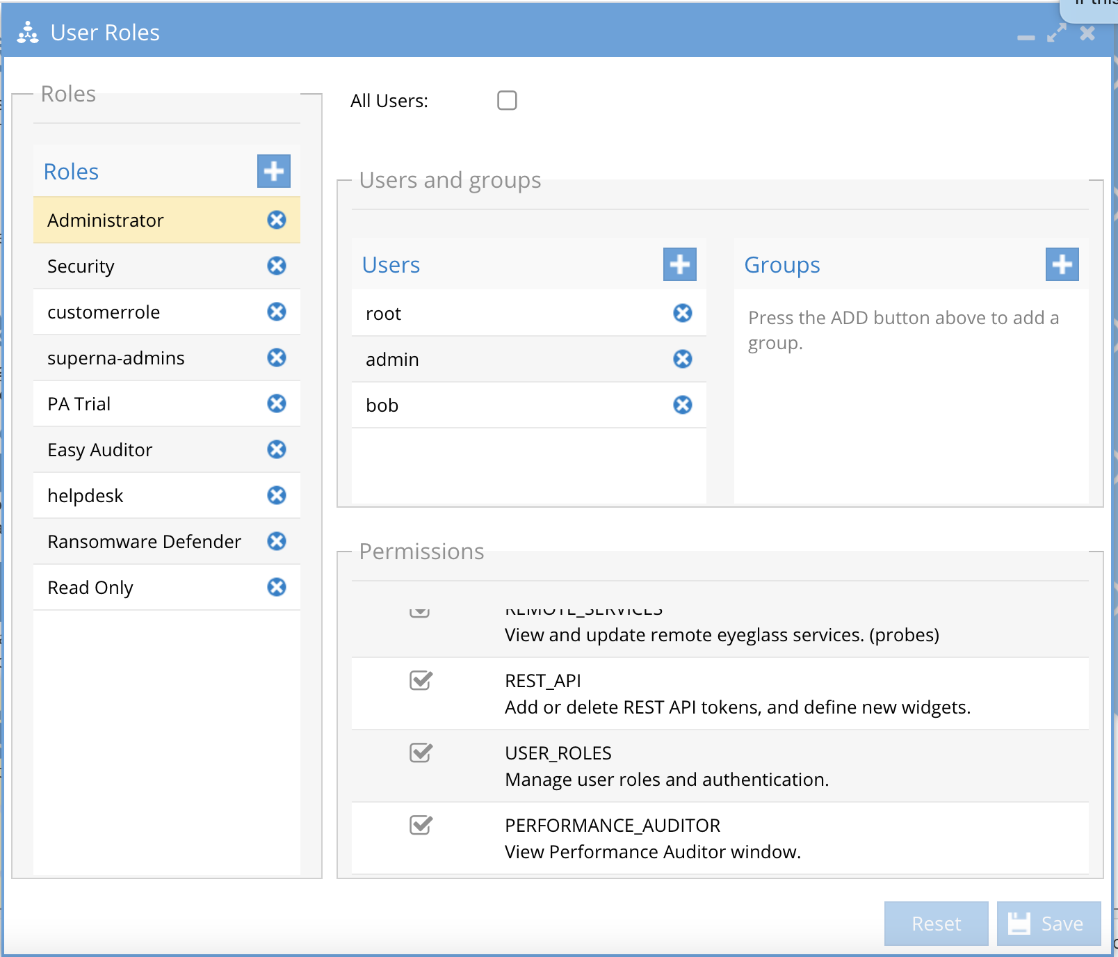
RBAC Role Required to Use Performance Auditor
- Release 2.5.6 update 2 20258 build or later
- The Performance Auditor icon will not display unless added to the administrator role or create a new role.
- The administrator role can be edited to display the new icon if a valid license has been applied. After adding the role and saving, you must logout and login again.
Baseline Performance Monitoring Overview
To understand performance it is important to know what normal performance looks like. This is possible with Performance Auditor's baseline Category Average feature. This feature will average all nodes, users, files, subnets and application extensions for read and write bandwidth to produce a cluster wide average. This average can be used to compare with the top 5 resources consumers in each category and see how high above the average the object is performing.
An average will not provide the best possible comparison, so Performance Auditor computes 2 positive and negative standard deviations above and below the average to provide a band that represents a more accurate average workload comparison.
How to use the Baseline Category Average
- Click on the Average indicator in the GUI to show the Read, Write and Total break down for the category total average. This can be used to compare to the top consumers and will display on the top right main performance display. Click Anywhere in the UI to unselect the Average indicator display in the top right of the UI.
- Now view the graph on the left to see the yellow shaded band that shows the full range of the average including the 2 standard deviations, this provides a more accurate view of the baseline average for the category.
- NOTE: The average is calculated across the same 60 second window as the top consumers in each category, so the comparison is the same time period shown for the top user, nodes, files, subnets and applications.
- See example average band below:
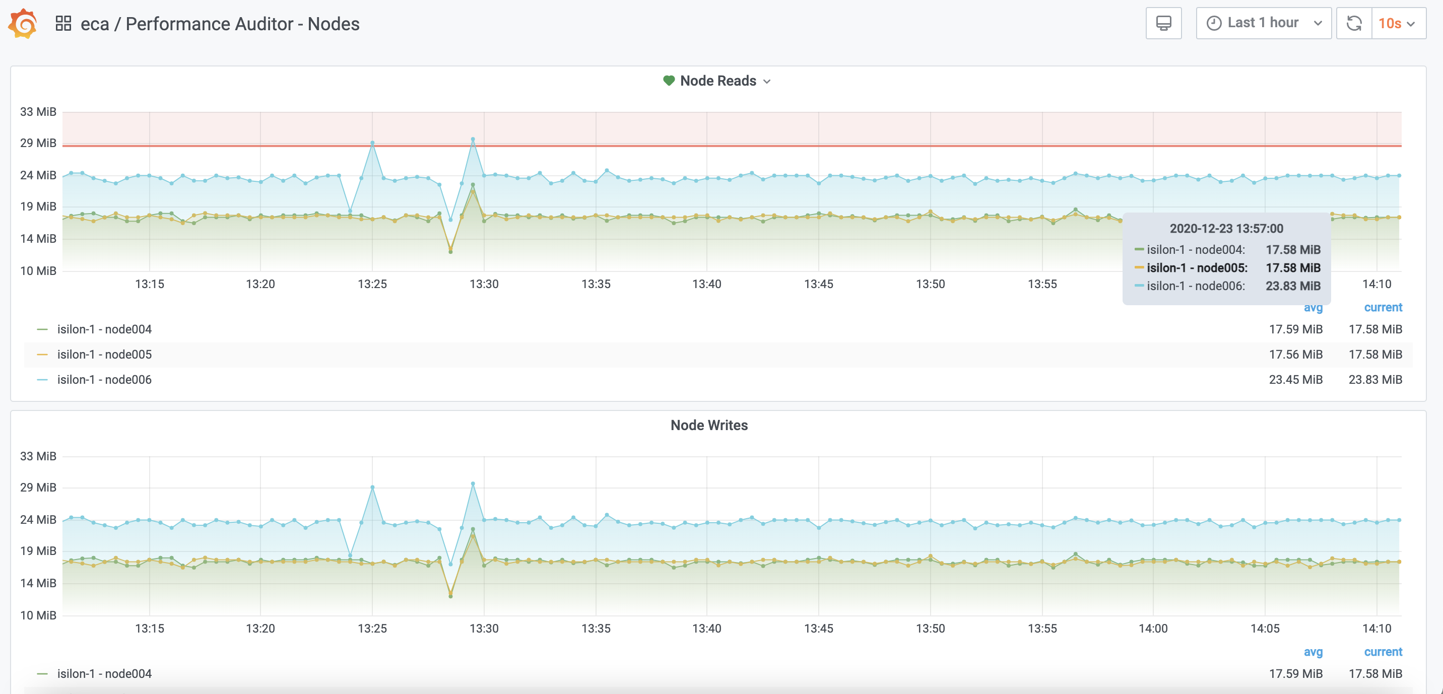
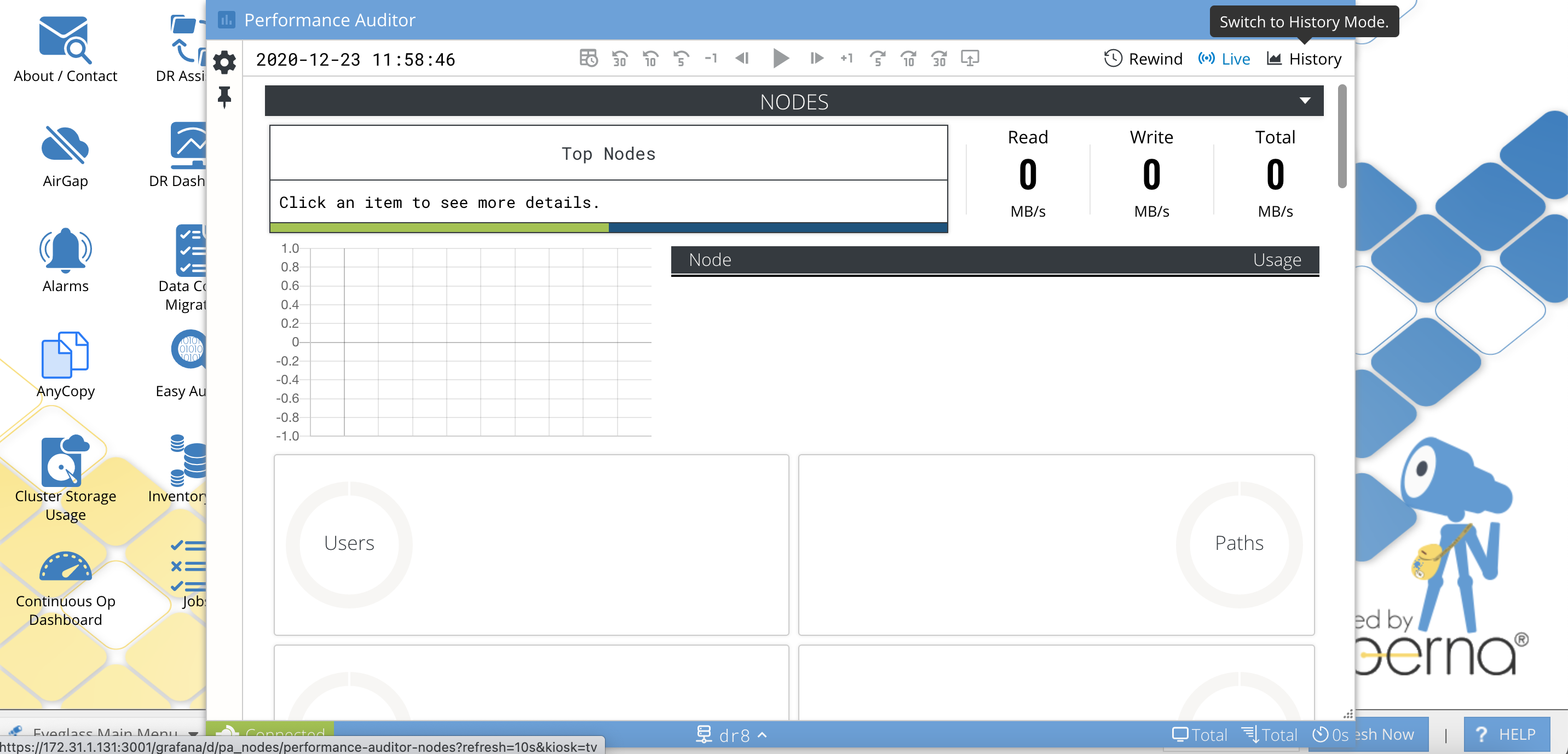
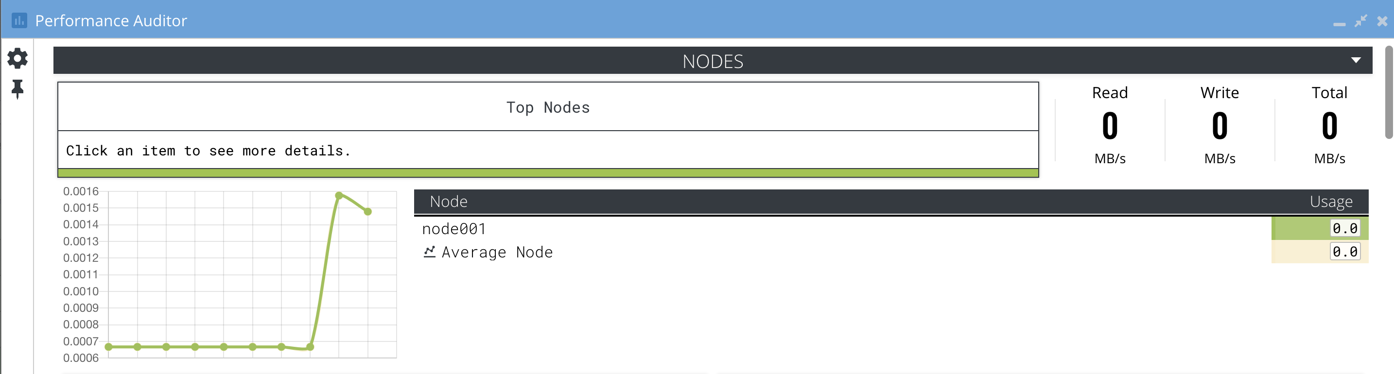
How to Trend cluster IO over time for the top cluster nodes
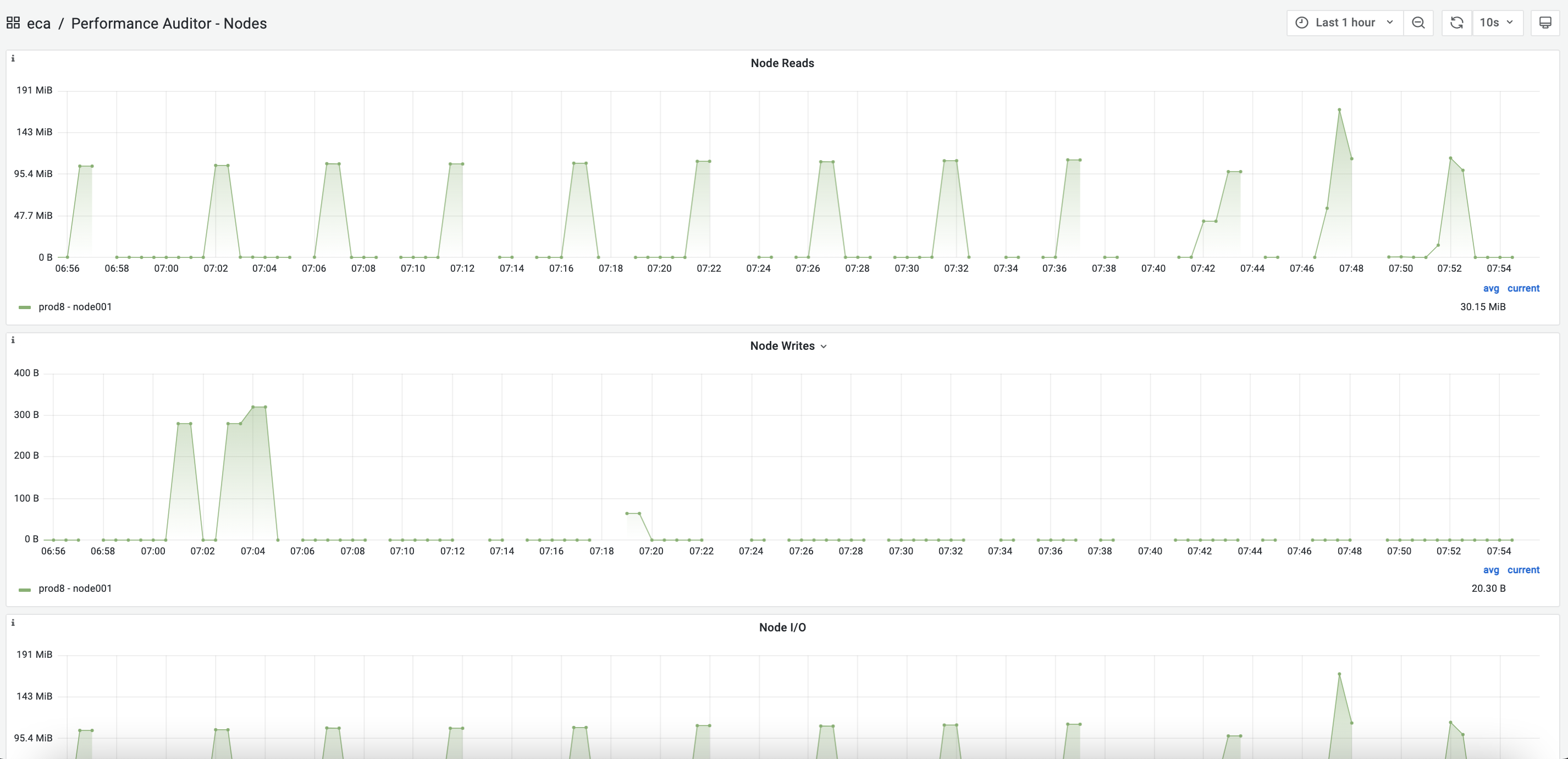
- New in release 2.5.7 is the history mode that provides a time series graph of historical cluster performance data.
- The history view can be accessed from the history link shown below.
-
- The graph below is an example of historical live data view
How to Use the UI
The interface uses views to show the performance data from cluster wide view that shows all nodes, users, paths, and subnets consuming read and write bandwidth IO displayed in KB's,MB's or GB's. The rate selector can toggle between MB's or GB's and is found in the top right of the UI.
How to Navigate the UI
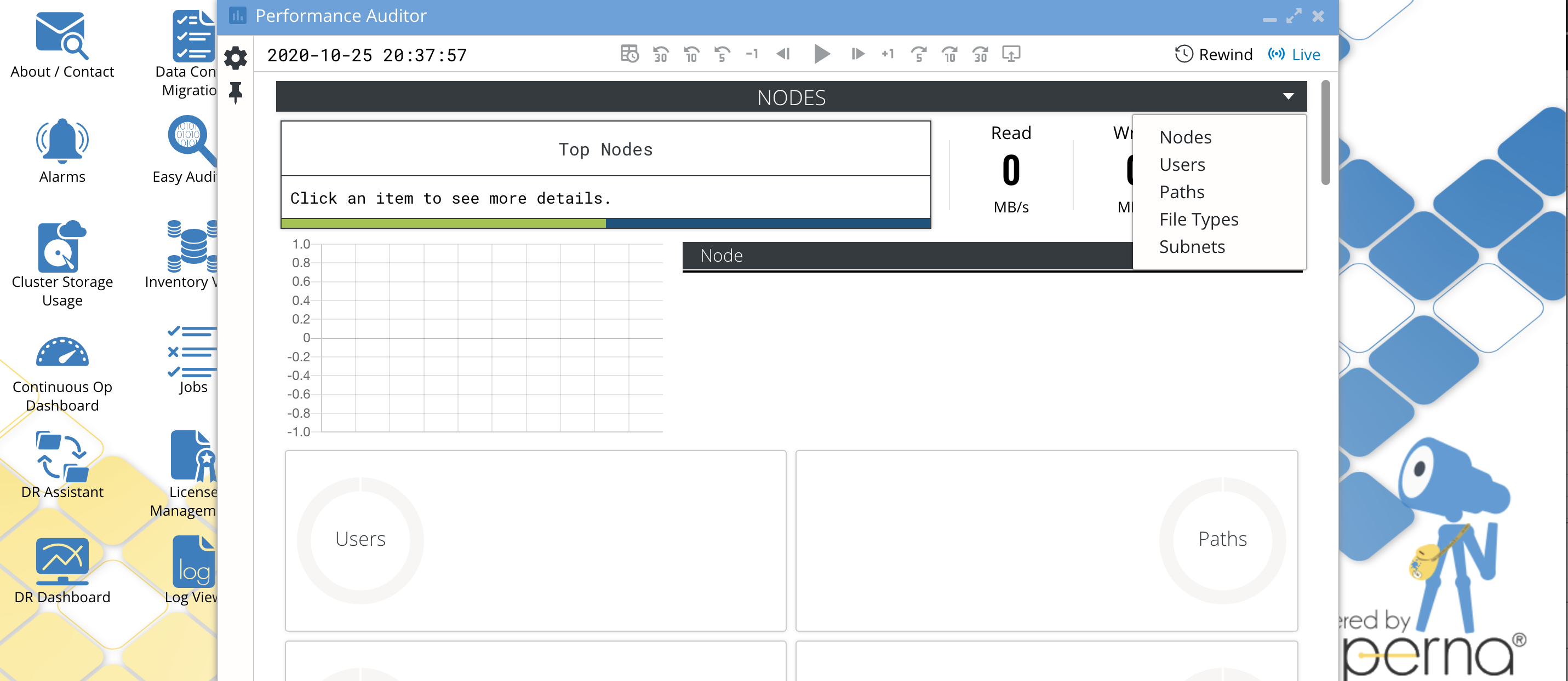
- How to switch between Vies (Users, Nodes, Paths,Subnet, File Types) using the drop down arrow on the top right of the UI.
- Select the rate in the settings icon.
- In any view select an object in the main window to show the specifics for the selected object below. Example in the default view selecting a node will dynamically show users, paths , subnets and file types that are consuming resources on the selected node. This concept applies to all views.
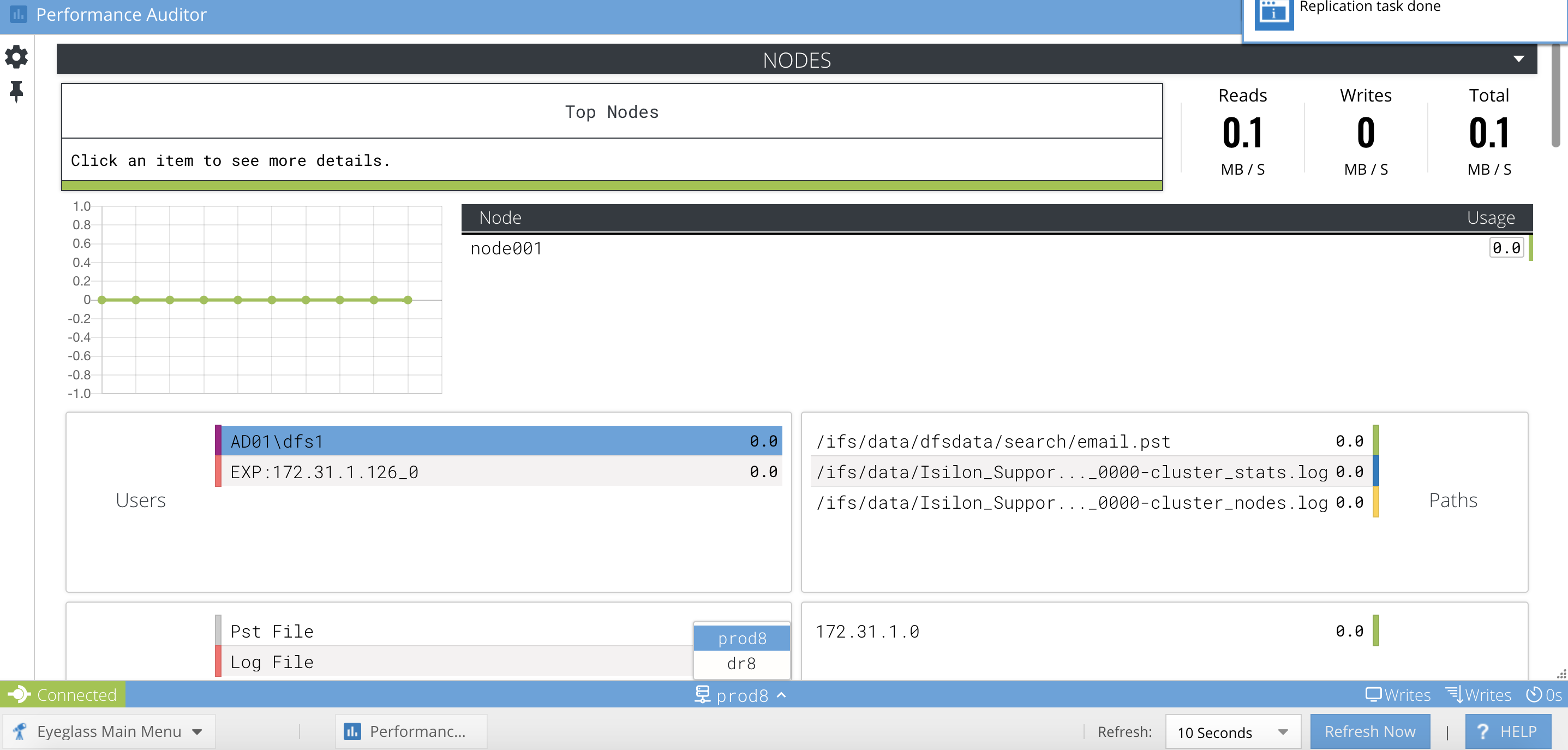
- By selecting an item in any view, anywhere in the UI will add the object to the Top box at the top of the UI (see example below). This allows viewing this object's performance with Reads and Writes bandwidth broken out including the sum of both for a Total.
- Performance Data indicator at the bottom of the Settings Window, shows "Connected" to the Performance collector and how long ago the "Last update" was revived by the UI. This tells you how current the data is that is displayed. Connected means the back end data source is providing performance data to the UI.
How to View Historical Performance data with the Rewind Feature
- The historical data is stored for approximately 14 days before it is auto deleted. This time range can be extended and will consume more disk space on the ECA cluster nodes.
- You can only view Rewind mode or Live mode at one time.
- Click the Rewind button at the top right for Historical mode or Click Live mode to switch back to current date and time.
- UI Controls
- The date and time of the data is shown at the top left of the display.
- Play pause button to stop playback or start again. Once it plays it will playback 1 second updates at the day and time selected.
- Select the Calendar button to pick a date and time. Once selected use the + - 1 minute, + - 5 minute, + - 10 minute and + - 30 minute button to fast forward or rewind through performance data to locate the issue.
- Once you have selected a day and time to view, you can switch views to see different category data nodes, users, paths, subnets and applications.

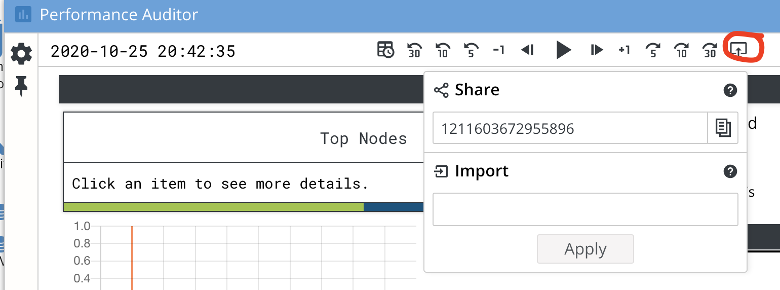
- Share a Day and time with another administrator or save a book mark. This Share mode stores the time series index number that can be copied to clipboard and saved to import and rewind to this exact point in time in the historical data.
- This can be shared with other administrators to view this date time and time by using the import option. Paste the number and click import.
How to view long term historical summary performance data graphs
- This data is stored in a time series database and allows graphing a subset of the performance data in an interactive graph.
- Access this historical graphs with the History link top right of the UI. This will open a new browser tab.
How to switch the UI display from one cluster to another
- At the bottom of the display in the middle you will see the cluster name that the Performance UI is currently displaying. Click the cluster name to see a list of clusters sending statistics from the ECA cluster. NOTE: NFS mount to the audit director is required before any performance data will display from a cluster.
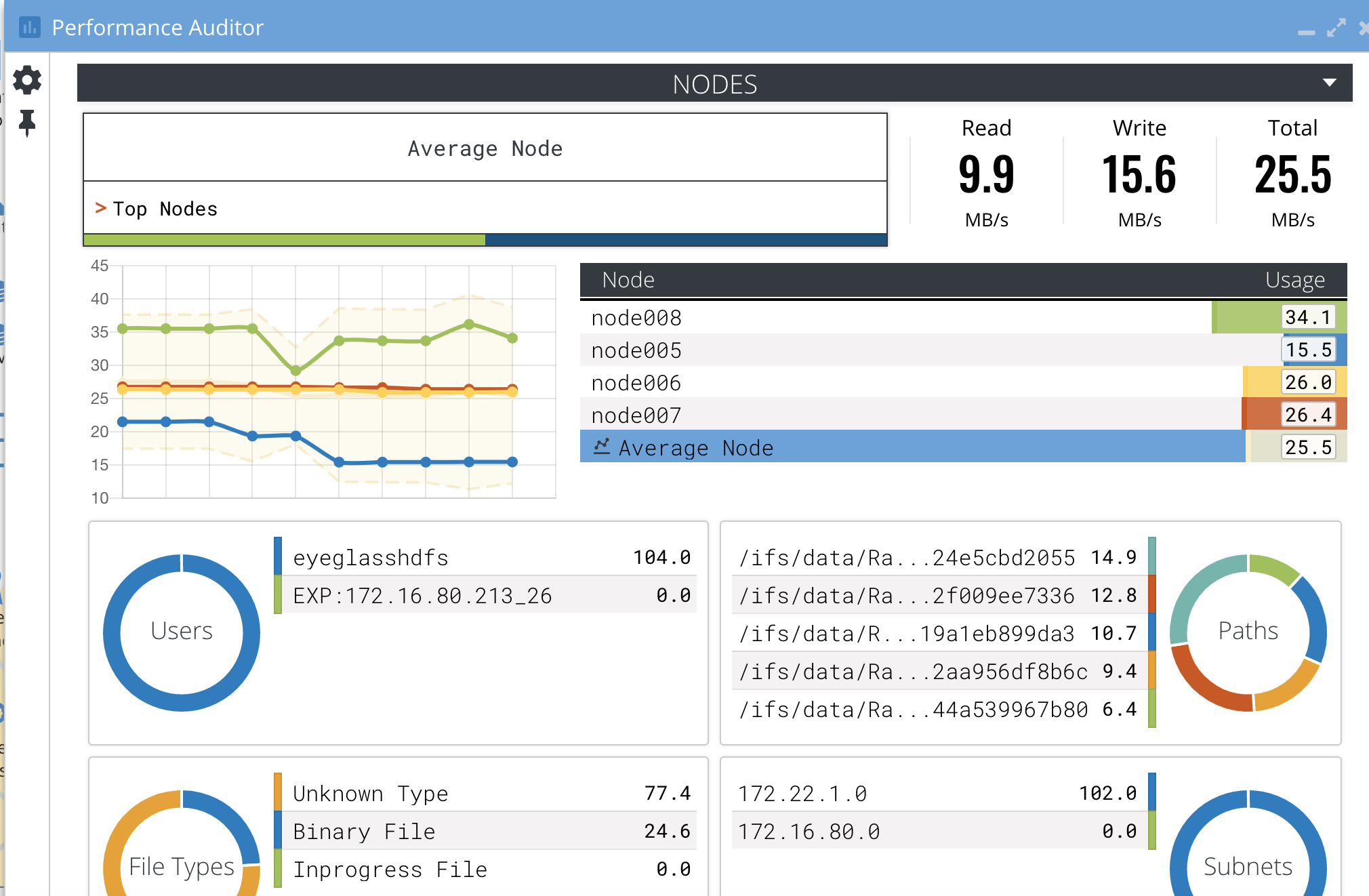
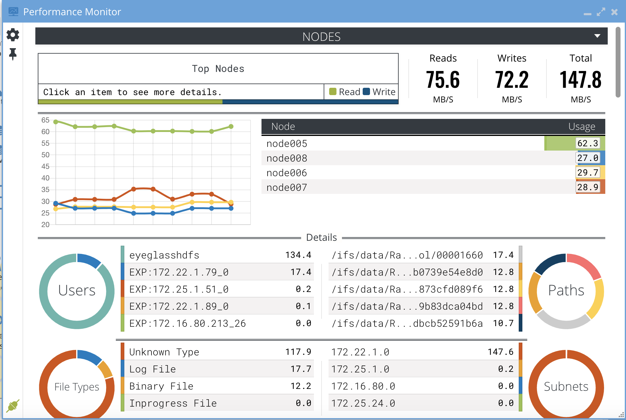
Cluster Wide Performance View Shows the Top Users, Paths, File Types, and Subnets and Category Baseline Averages
NOTE: The Average Category stat is an average for all items and not just the top 5 resource consumers displayed in the UI. Example the nodes average is all nodes in the cluster averaged over the last minute to allow comparison to the top nodes in this view.
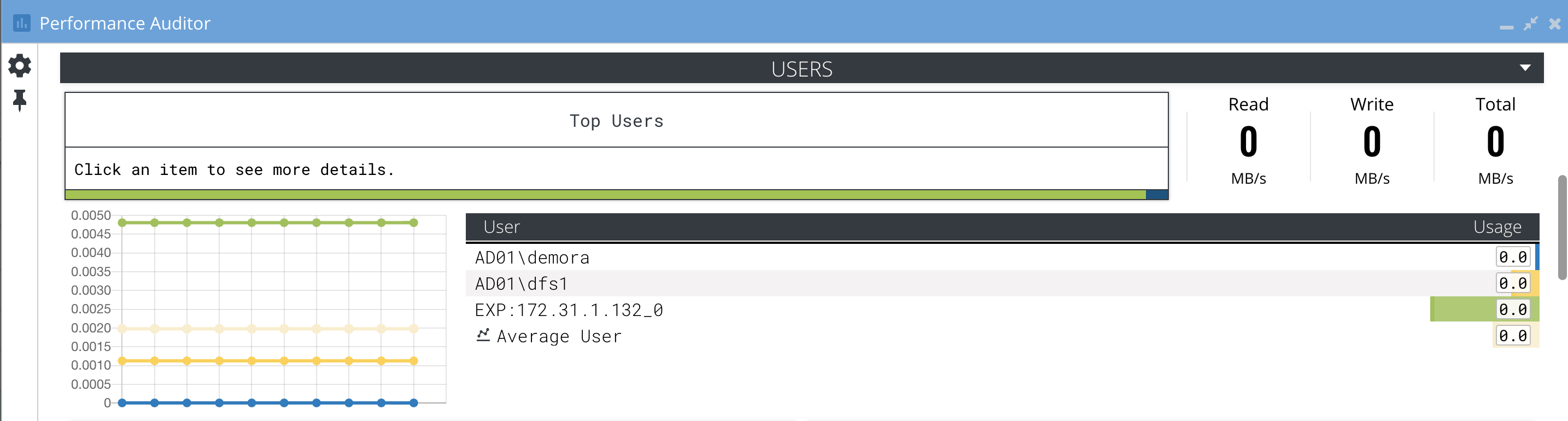
User View shows the Top Users with Baseline Average and Nodes, Path, Subnet and File Types breakouts below
Path View shows the Top paths with Baseline Average and node, user and subnet breakouts below

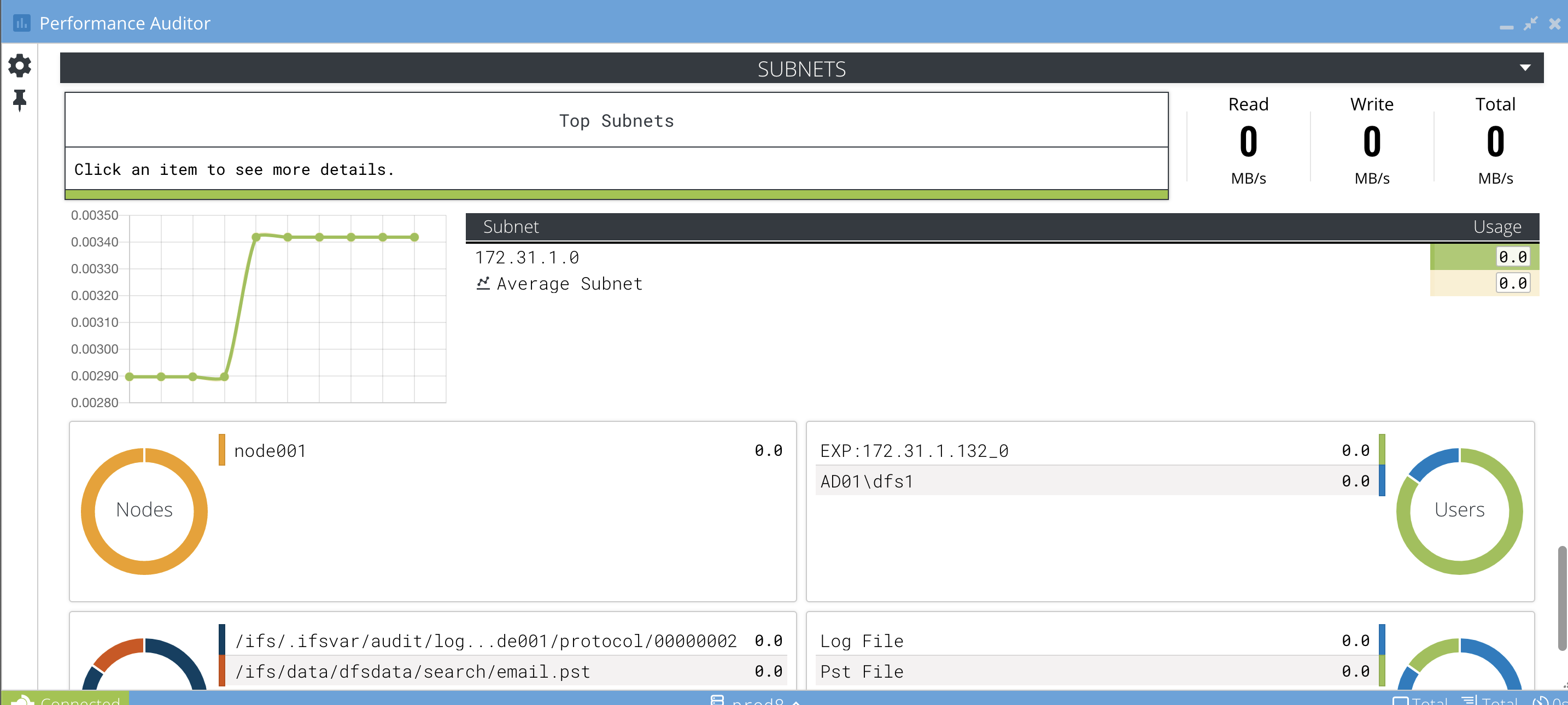
Subnet View shows the Top subnets with Baseline Average and nodes, users, and paths breakouts below
NOTE: Subnets shown are based on all source IP's of IO across the cluster nodes with a /24 subnet mask applied to show a break down by subnet. Performance Auditor has no way to know what the actual subnet mask is for your network. This view provides a relative break down of source IP's, use this view and combine this data with your knowledge of the actual subnet masks in your environment.
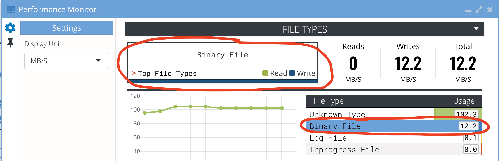
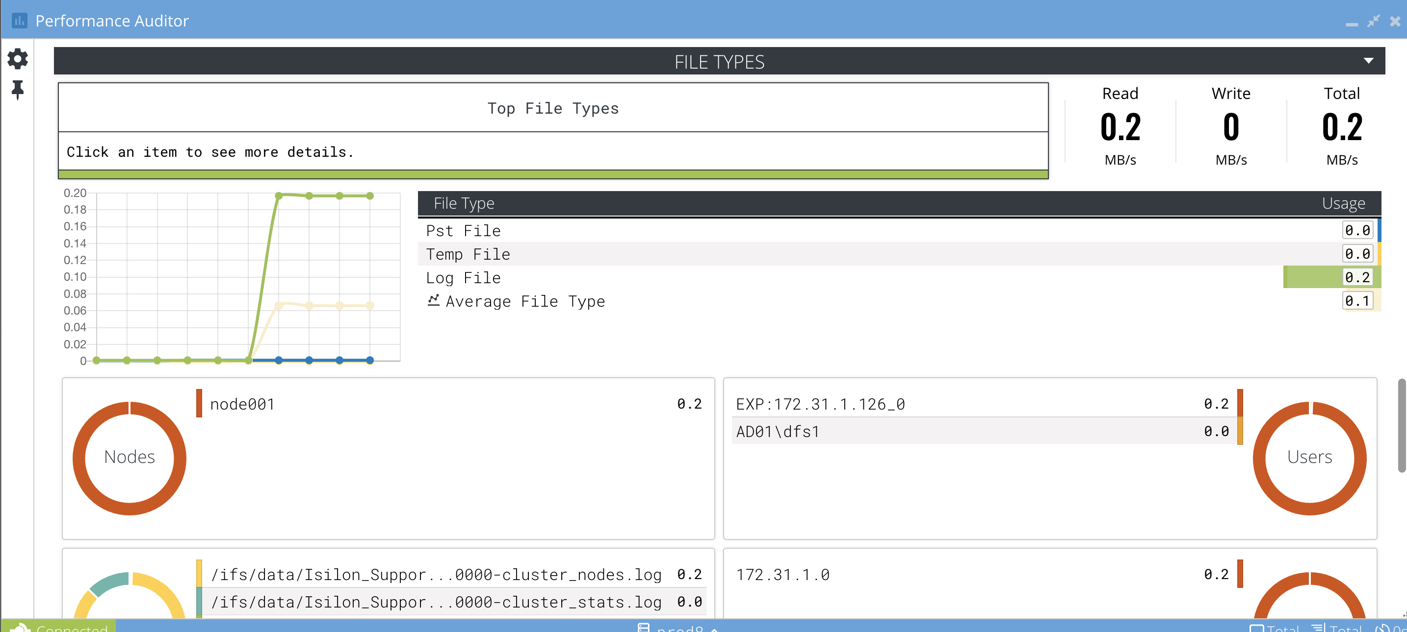
File Types View Shows the Top application types with Baseline Average and nodes, user and subnet breakouts below
How to change the throughput rate shown for all Views
- Click the Settings icon.
- Sort each performance category using the sort by option.
- Unclick the "Compute average rate over 1 minute" to switch to MB committed per minute versus the rate of throughput calculation.
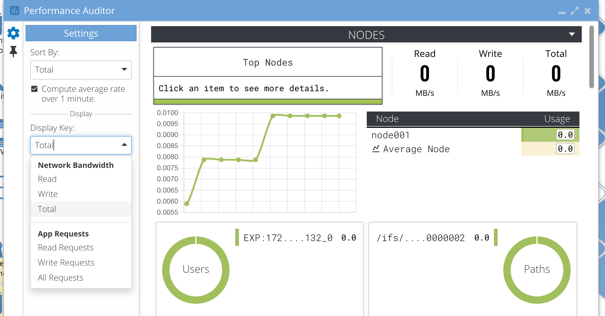
- Use the "Display Key" drop down to change the display rate for Reads, Writes or Total, and “Units” to select KB, MB or GB per second rate display in all UI's.
- To switch the category display to show the Application Requests per second select All Requests under app Requests.
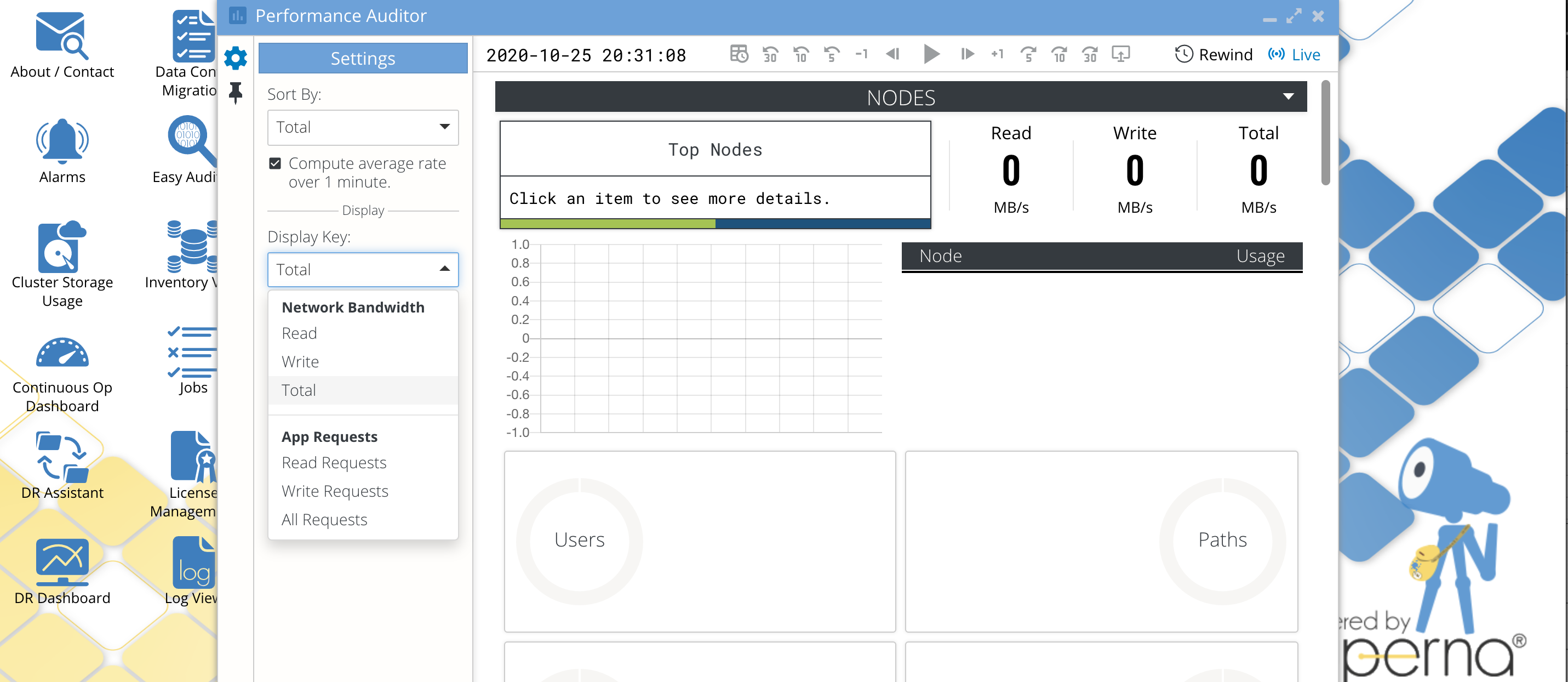
How to Switch to Application Requests Statistics
- Click the Settings icon and select the "Display Key" drop down and select "Application Requests". All displays will now show Application Requests per second. This is similar to IOPS but is application specific IO read, write or total application requests per second over the last 1 minute sample window. This provides insight into the application IO patterns and how often the application commits data on a write or how much read ahead is being done by the application.
- Example: A higher rate of application requests means smaller IO requests and less tolerance to network latency since more round trips are required with each application commit for a write or reading data many times per second vs caching data locally and larger reads.
- Set the Display Key to read, writes or total to show that stat in each category view. Example to show Reads for all nodes set the Display Key to "Read" and now all nodes will show Reads for the value in the top 5 list for each area (nodes, paths, users, subnets, applications)
How to trouble shoot by Pinning Users, files, nodes, subnets to Performance Views
- Use Case: A common issue is a complaint of performance issues by a user or application using NAS storage. The pinning feature is designed to allow focusing on a node, user, file or subnet to the display how it compares with the top five resource consuming aspects of the cluster.
- NOTE: You can only pin 1 object in this release
- Example #1 User with performance issue is sharing a node with a backup application that is creating large files and using most of the node resources.
- Example #2 a top 5 user is visible in the GUI and you want to continue to monitor this users file performance. Pinning this user to the display will keep this user's files and statistics in the display to compare to other users nodes subnets etc.. Without pinning the user may disappear from the top 5 list.
How to pin a User using with Drag and drop
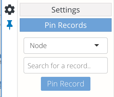
- Click the Pin on the left side of the UI:
- Select the User View:
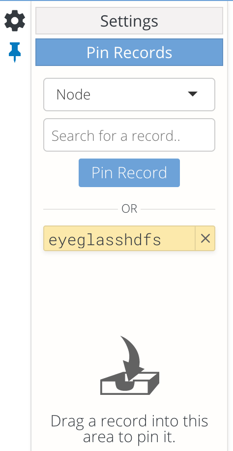
- Drag the user from the main view over to the pin record area. It will display the pinned user:
- You can hide the pinned view by clicking on the pin icon.
- NOTE: The pinned record will only be visible on the View for the record type. For example pinning a user will display on the user view, pinning a node will display on the nodes view. You can select any record type on any view to pin the record but the pinned record is only going to stay on the record type view.
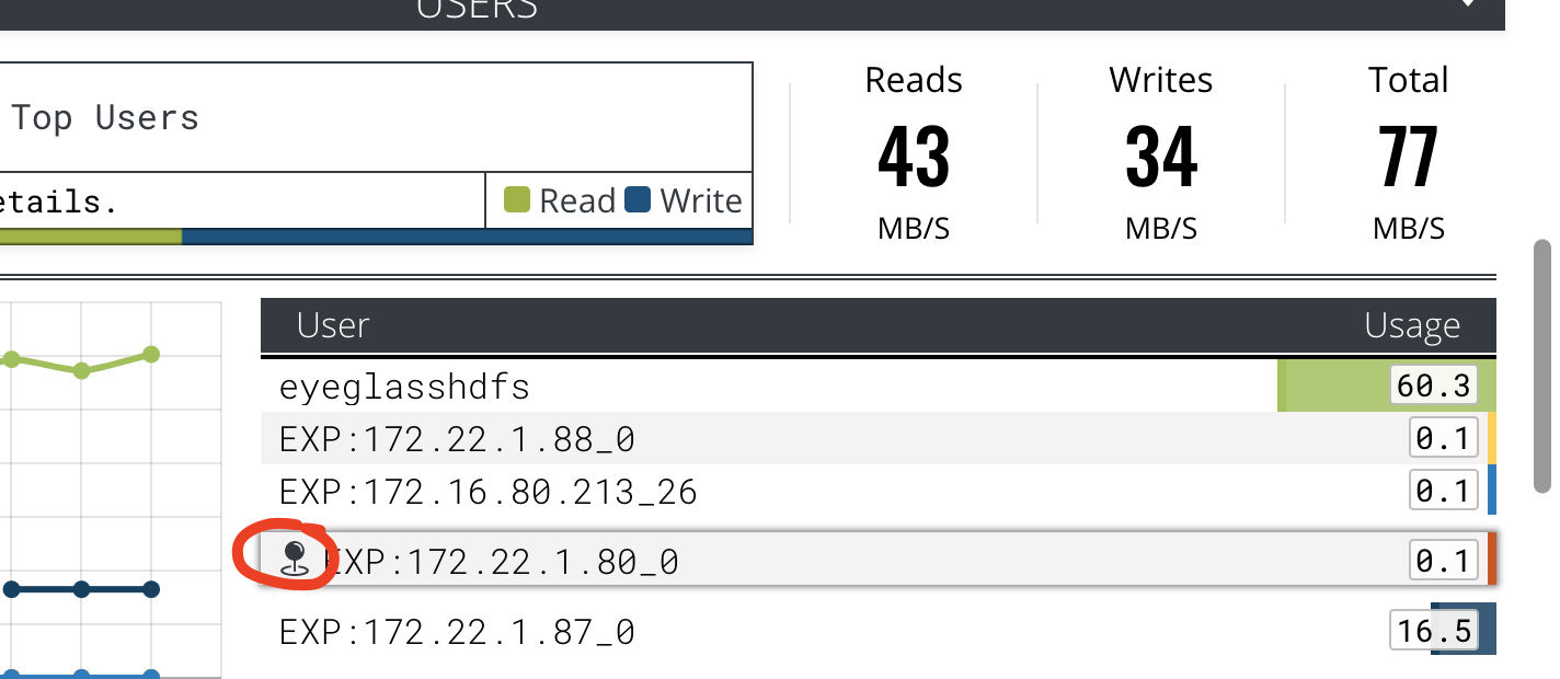
- Once pinned an icon indicates the record has been pinned which means it may not be a top resource consuming record but is pinned to the display for comparison to other records within the view. This allows you to monitor the record (user, node , file type,, subnet, file).
How to remove a pinned Record
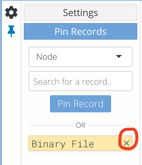
- Click the pinned icon on the left side of the UI.
- Click the X next to the pinned record:
How to add a pinned record for a user, file, subnet, node application type not displayed in the UI
- User Pinning example:
- Click the pinned icon.
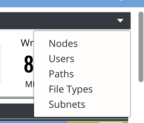
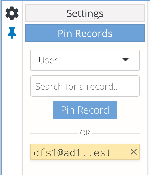
- Select the record type selector drop down and select "User".
- Enter the user with "user@domain.com" syntax.
- If the user is resolved to a SID correctly it will be added to the display. If the user is not resolved you will receive an error message after a timeout "Error: Username 'xxxxx' could not be resolved."
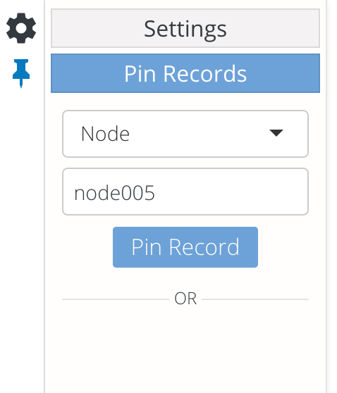
- Node Pinning Example
- This option allows you to add a node, not listed in the top 5, to the display, and compare its usage to that of the top 5.
- Type the name of the node using the syntax shown similar to other nodes listed in the active view.
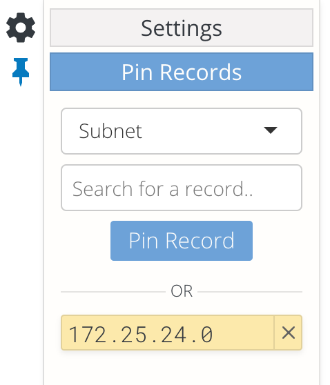
- Subnet Pinning Example
- For Subnets use the drag and drop method or enter x.x.x.x and assume a slash 24 subnet or 255.255.255.0.
- Select the "Subnet" from the drop down and enter a subnet record example 172.25.24.0 this will grab all IO in the 172.25.24.0/24 subnet to display.
- How to enter your own subnet: Simply enter the first 3 octets of your subnet and .0 at the end to collect all the hosts in that match 255.255.255.0 default subnet matching logic.
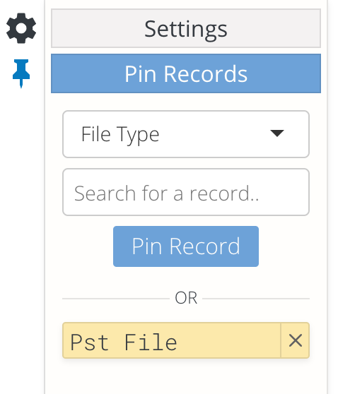
- Node Application Type Pinning Example
- For application pinning select "File Type" option in the drop down menu.
- Enter the extension (i.e. pst will monitor all pst file IO across the cluster).
How to enable MB committed mode for long running file copy application use cases
- This can be found in the "Settings" icon at the top left of the user display.
- This feature switches from rate based measurement to commented data per 60 second window, which captures long running file copies or applications that creates very large files and take longer than a minute to create.
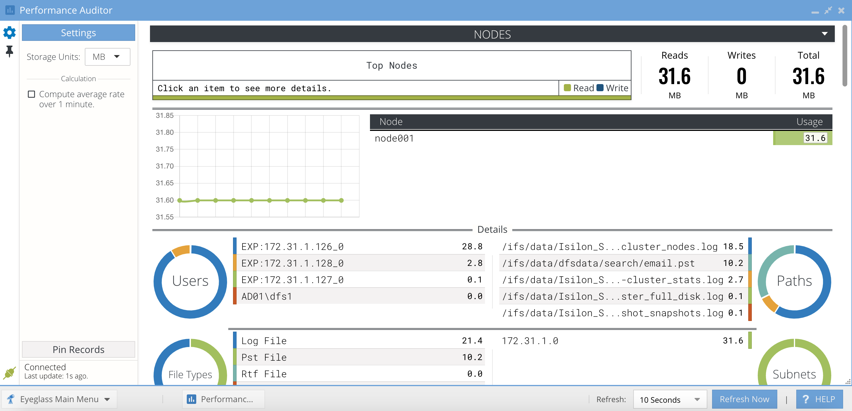
- This will toggle all displays to show total MB of data committed per minute, which is another metric for load on nodes when applications commit data at the end of the create logic. This is true for many large file copies or similar new file create work loads like video rendering. This metric is not rate based but shows the total MB's committed by applications over the last 60 seconds .
- The example below shows 31.6 Total MB were read in the last 60 second sample window. Each 1 second update is the total Sum of all files that were committed to storage.
How to Enable MB per minute committed mode
- Click the Settings gear icon.
- Uncheck the "Compute average rate over 1 minute" check box.
© Superna Inc